
Visualizing What You (Should) Already Know About RB Production

Nietzsche killed God. Factories started burning coal. It was game over for community. It was just the beginning for men like us.
- Whitney Halberstram, Industry (TV)
Welcome back, friends. Judging by the subscriber data map I have available to me, Substack tells me that a large percentage of you are located along the East Coast of the US and Canada. BRRR!! 🥶
I hope you are somewhere warm and cozy currently, if that’s your jam. Personally, I’m a Winter soul, and so later this afternoon, I plan to dust off my explorer’s hat and attempt to skate on the frozen bay around Toronto’s islands. Wish me luck!
Now, if you’re already subscribed to this publication, then you’re already well aware of the connection between volume and production in the context of college football. A player can’t score if he doesn’t have the ball in his hands. It’s a simple concept. And the best part is, it’s actually probably easier to predict volume than it is to forecast output.
I think one of the first revelations for any new College Fantasy Football (CFF) player is that there are a lot of factors that determine which players are the most productive.
Conventional (casual) sports fan wisdom deems that the players with the most stats are the best. However, these fans fail to account for the system that the player plays in. Namely, how many opportunities they receive (more on this shortly), the efficiency of other players around them, quality of play from position groups they depend on (i.e. OL play for RBs/QBs, QBs for WRs) etc.
We spend a lot of time here at this publication attempting to predict which players will see the most touches each season. In fact—dare I say—I may be the single world leader in time spent thinking about where carries will be distributed in college football (and I don’t claim this proudly).
When it comes to opportunities and how they are distributed in college football, there is nuance involved. The scope of this analysis does not attempt to answer the question of why players receive the opportunities they do, rather, it is to reinforce what most readers already know about the relationship between input volume and output.
But I will offer a few thoughts on the question anyways. Of course, there is a relationship between player ability and the opportunities he receives. The players who are deemed to be ‘better’ by a coaching staff will oftentimes receive more opportunities. When one player absorbs 70% of a team’s rushing carries, it is reasonable to infer that the staff have judged that player’s ability to be higher than the other players in the room at a minimum.
But it is also just the case that there are coaches who have sticky preferences regarding how they want the touch distribution to look in their backfields.
For example, there have been a lot of good RBs at the University of Georgia under Kirby Smart. However, none of them post-COVID have finished with a PPG average over 20. In fact, most don’t even reach 15.
Indiana have run the ball very effectively under Curt Cignetti for the past two seasons. If they consolidated touches primarily to one RB, there’d be a monster CFF asset there. But they don’t, so their RBs are not relevant.
In contrast, there are coaches with offences that systematically distribute 50% or more carry share to the RB1, e.g., Minnesota’s PJ Fleck, former OKST coach Mike Gundy, former SDSU coach Rocky Long in the 2010s, former Wisconsin coach Paul Chryst in the 2010s, current Arkansas QBs coach and former Marshall/JSU OC Clint Trickett, Texas’ Steve Sarkisian, ULM’s Bryant Vincent etc.
To that end, the coaches that a player plays for may actually be the single most important factor in determining how many carries he will receive, and by extension what his output will be (perhaps even more so than how good he is!).
Though there are also examples where an individual player’s talent supersedes the desired philosophy of the play caller (e.g., Emmett Johnson at Nebraska, Daylen Smothers at NC State, Demond Claiborne at WF in 2024 etc)… and sometimes it’s just as simple as being the last man standing in a room (I’m going to start referencing the last man standing theorem in future articles).
In short, the practice of predicting player volumes will never be done with scientific precision. But maybe this topic can be another stand alone article I work on in the future.
Anyways, with the help of my new friend ClaudeAi, and Fantrax’ downloadable data, I have prepared some visuals for the reader to confirm some of the things we believe in regards to the game of CFF.
The data is a stored in a public Google sheets document for your reference (it’s just a CSV downloaded from Fantrax). A sample of the top 100 rushers by PPG (1PPR) is selected. From a CFF perspective, this group captures most of the relevant players in a given season assuming a normal 12 team league with somewhere between 16 and 24 players rostered each. Though I will note in the article where limitations occur of working with a small sample like this.
Plot 1. CARRIES VS. RUSHING YARDS
As you should expect if you’re a reader of this publication, there is a clear positive relationship between carry volume and rushing yardage. Every player that cleared the 235 carry threshold, for example, ran for over 1000 yards in 2025. In fact, if it weren’t for former CAL and current SMU RB Kendrick Raphael’s poor performance, every RB with at least 212 carries cleared 1000 yards.
In contrast, every player with less than 140 carries failed to rush for 1000 yards, and only two players with less than 150 carries hit 1000 yards rushing.
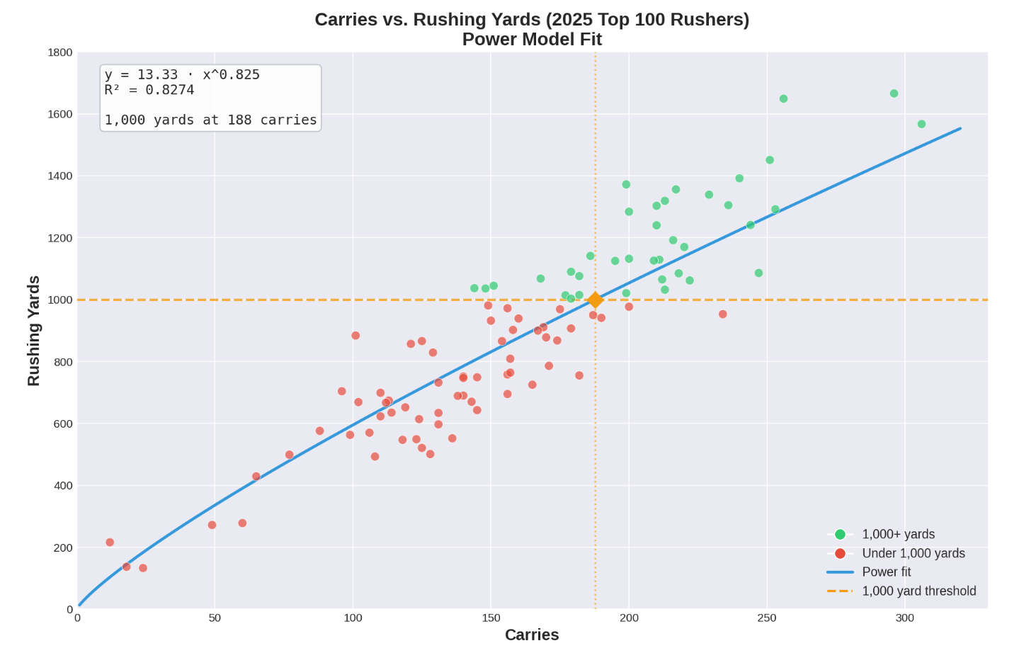
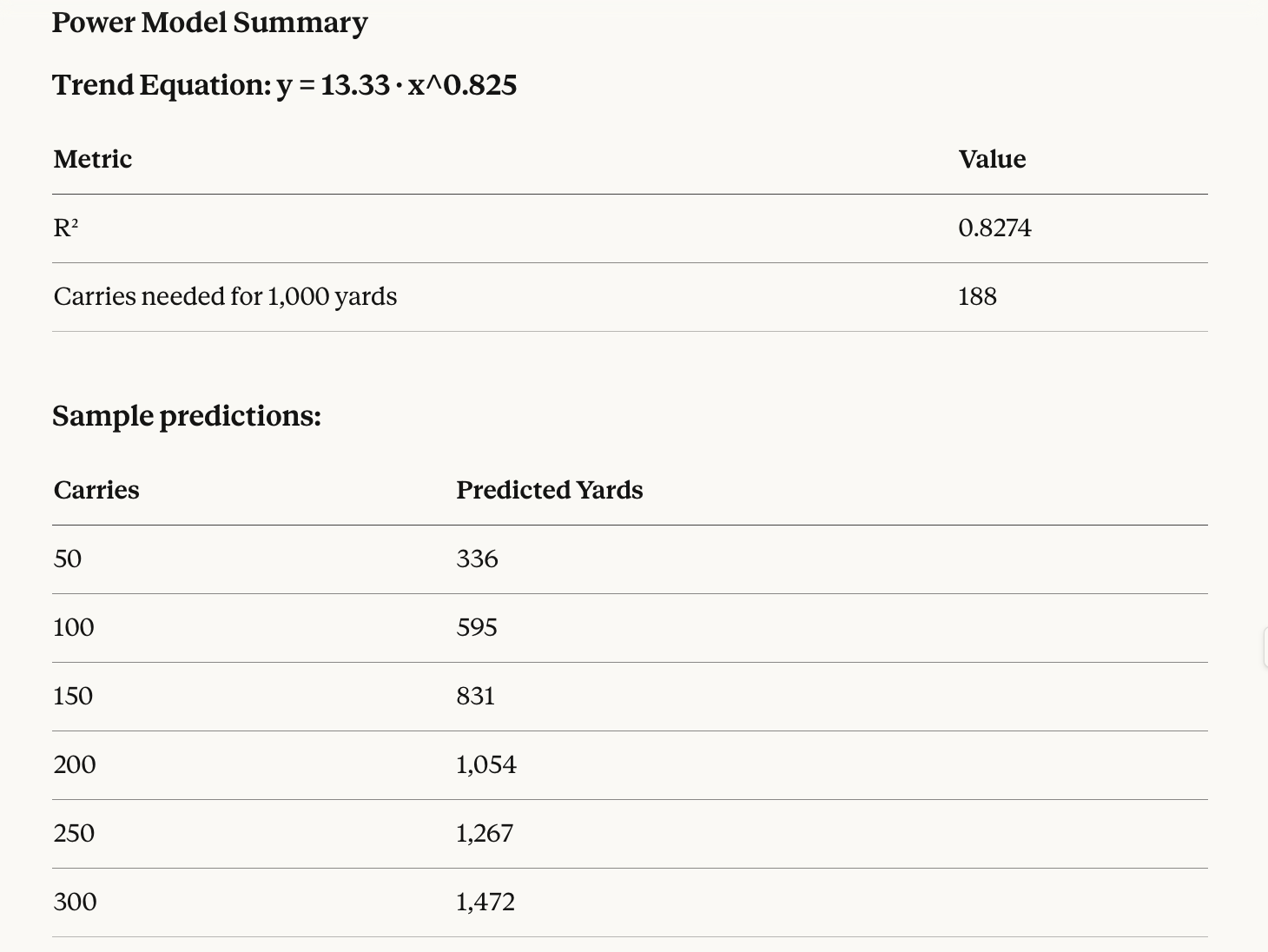
The model predicts you need 188 carries on average to hit 1000 yards—which aligns reasonably well with what we see in the data (most players hitting 1000 have 180+ carries).
Even though we have only a sample of players from one season, I actually think this threshold would prove rather robust in a larger sample size with minimal variation.
BTW—why a power model to fit this data?
It allows for a measure of diminishing returns on higher workloads. The exponent of 0.825 (less than 1) confirms diminishing returns amongst the sample—each additional carry contributes slightly fewer yards than the previous.
This reflects the effects of fatigue, defensive adjustments, and lower weighting on each individual per carry (e.g., one large run can heavily skew YPC average in a smaller in a workload relative to a bigger one).
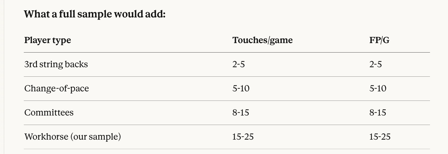
I’d imagine that in reality there is probably a sweet spot, where less than say, 10 carries in a game, is not good for accurately assessing player ability (players need to get warmed up, remove jitters, etc), and over 25 carries is probably where 90+% of players will begin to degrade in performance (this is just me spitballing, there’s no modelling behind this 90% number).1
Keep in mind that the sample this program is using is the top 100 rushers from 2025 college football by yardage, so there's going to be some sample selection bias that is putting upward pressure on the efficiency in the model.
The ‘a’ value in our equation here is 13.3, which sets the scale of the curve, and is what would translate up and down with different efficiency. A less efficient group of RBs would have a lower ‘a’ value. The shape of the curve would still look the same, but it would commute a few notches lower from where it is now.
Hypothetically, if I were to train the program on the next 100 rushers by yardage, I would expect the value in the trend equation to be lower than 13.3, because I would expect that the top 100 rushers are on average more efficient than the next 100 (while systems are a tried-and-true method to predict volume, better players also earn more touches), but that could be a flawed assumption.
In fact, the more I think about it, maybe it is! Those with lower yardage are also likely to be seeing fewer carries, and thus their YPC averages may actually be… higher on average? Why don’t we verify this assumption?
I asked Claude to perform a hypothesis test on whether the top 100 rushers were more efficient than the next 100 rushers.
Hypothesis Test
Hypothesis: The top 100 rushers are more efficient (higher YPC) on average compared to the next 100 rushers (ranks 101-200).
Results
Top 100 Rushers (Ranks 1-100)
Average YPC: 5.52
Median YPC: 5.55
Standard Deviation: 1.09
Next 100 Rushers (Ranks 101-200)
Average YPC: 5.07
Median YPC: 5.10
Standard Deviation: 0.98
Difference
Difference in Means: 0.45 yards per carry
Percent Difference: Top 100 are 8.9% more efficient
Statistical Significance
Two-Sample t-test Results
t-statistic: 3.14
p-value: 0.0018
Result: STATISTICALLY SIGNIFICANT (p < 0.05)
Conclusion: The difference in yards per carry between the top 100 and next 100 rushers is statistically significant according to Claude. We can reject the null hypothesis (i.e. there is in fact a difference in efficiency between the top populations) and confirm that the top 100 rushers are indeed more efficient on average.
Ok, I’m glad we got to the bottom of that.
So, we’ve briefly studied the relationship between carries and rushing yardage for college football’s leading rushers, but in today’s game, increasingly a player’s value derives from their ability to provide value in the running and passing games. And ultimately, what CFFers covet is a player’s PPG output.
With that in mind, we can see below the relationship of total touches (carries + receptions) to points per game from the same group of 100 rushers.
Plot 2. TOTAL TOUCHES vs. PPG
Total touches is recorded as carries + receptions, and plotted vs. the players’ PPG (full PPR). The below plot shows both the power curve, and the linear curve.
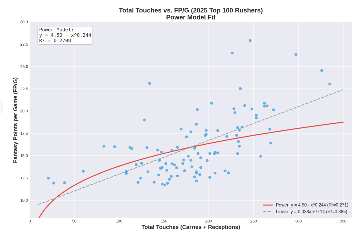
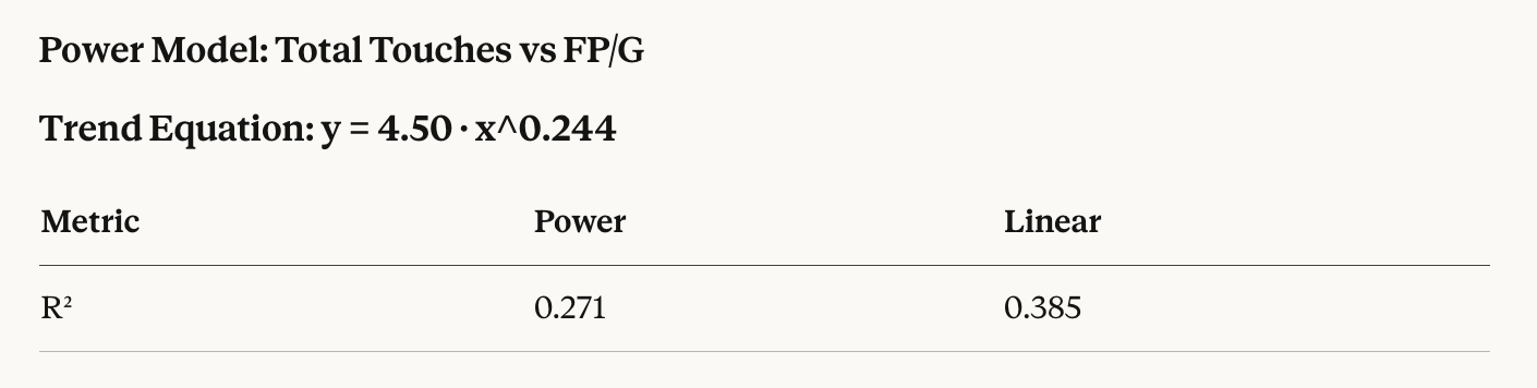
Look at the linear regression trend equation below—can you see why the linear curve is not appropriate for this data set? Hint: plug in one touch for ‘x’ in the equation below and see what PPG is expected of that player…
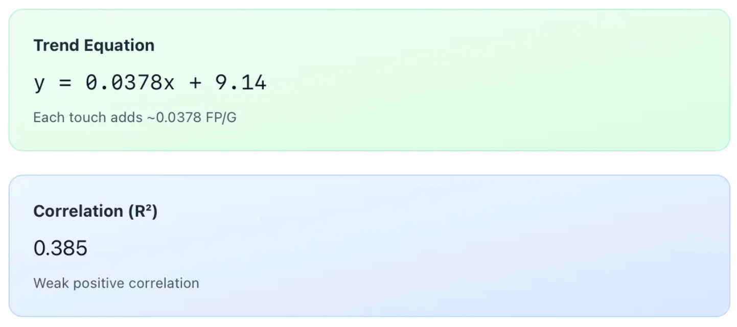
To map the linear model appropriately, the sample of players needs to be much larger, so that there are carry volumes represented at each level, including zero.
Yet, it is fair to say that linear curve actually fits the data much better than the power curve. The plot also suggests that touches only display a moderate to weak correlation to PPG (R squared value is 0.271). Hmm… I’m not convinced.
And if you’re not convinced either, there is a good reason. Plotting total touches vs. a per game stat like PPG is a faulty method to establish this connection.
There are players who suffered an injury during the season, and thus their total season touch figure will be unimpressive, yet their PPG average may still be elite (think players like Justice Haynes, UM, Waymond Jordan, USC etc).
Furthermore, many of these players would not show up in the group of top 100 rushers by rushing yardage (someone like Desmond Reid, perhaps), so the sample is limiting us here.
Nonetheless, a better way to do this would be to first compute the touches per game averages of this data set, and then plot vs. PPG.
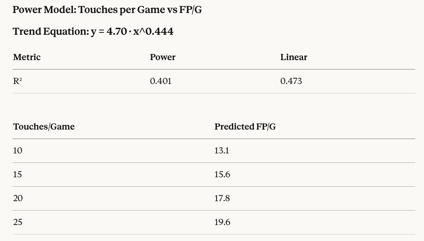
Plot 3. AVERAGE TOUCHES vs. PPG
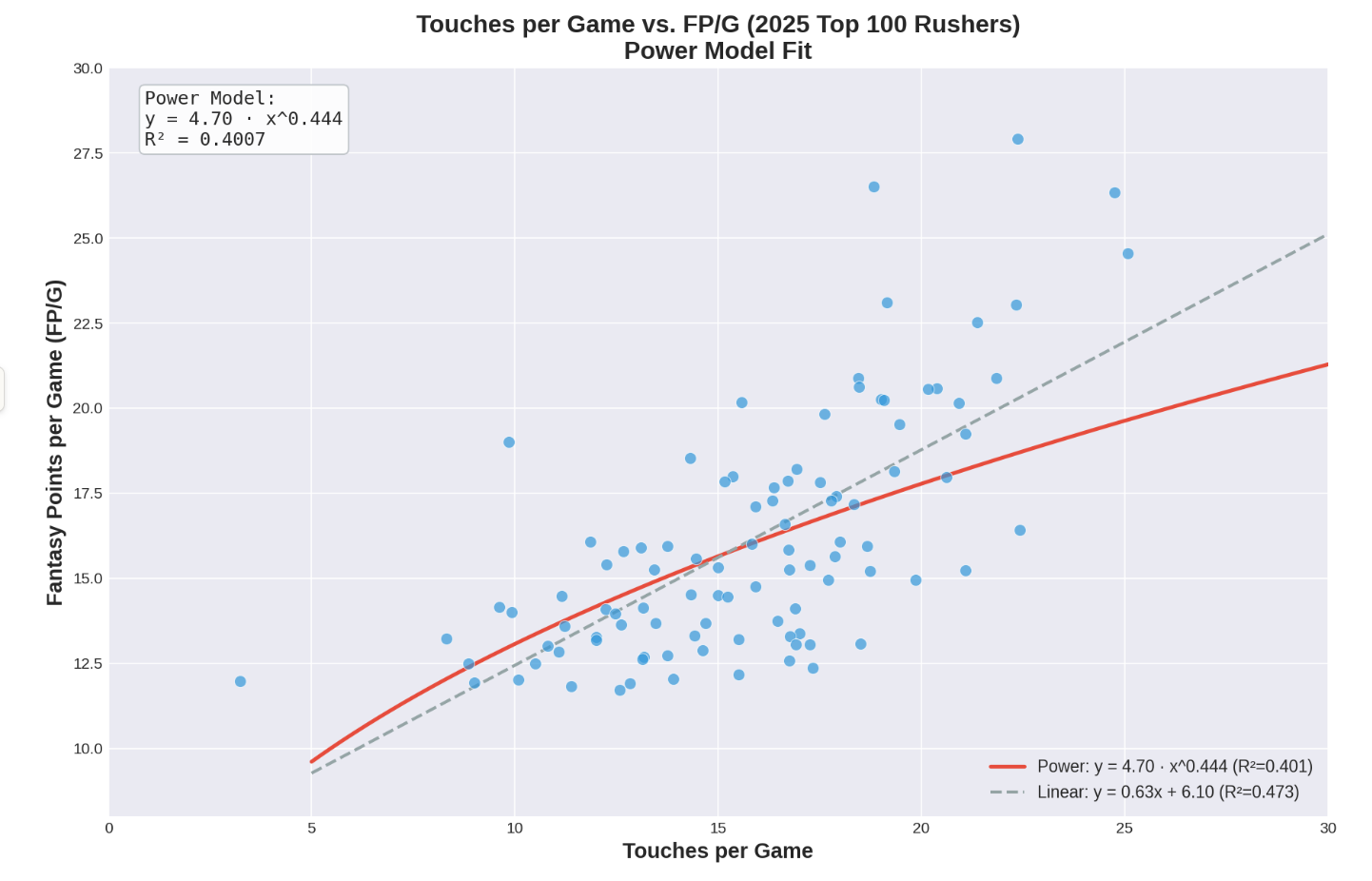
Observations of the updated plot:
Much better fit than total touches (R² jumped from 0.27 to 0.40/0.47)
The exponent (0.444) is much lower than the carries vs yards model (0.825), indicating stronger diminishing returns. This makes sense—going from 10 to 20 touches/game doesn’t double your fantasy points because:
Touchdowns don’t scale linearly with touches
High-volume backs may face stacked boxes
Efficiency tends to drop with extreme workloads
Still ~50% unexplained variance—other factors matter a lot: touchdown luck, how much of the usage is receiving usage, player efficiency, game script, etc.
Current sample bias:
Our top 100 by yardage is a narrow slice of successful, high-volume backs. They’re clustered in a relatively tight range:
Touches/game: mostly 12-22
PPG: mostly 12-22
This compressed range makes it harder to detect a strong linear relationship—we’re essentially zooming in on a small section of the curve where noise dominates.
With a full range of RBs, we’d see a much clearer trend from the bottom-left to top-right of the plot. The relationship “more touches = more fantasy points” would be obvious.
Model fit and sample bias aside, one key takeaway of the relationship between per game volume and PPG is clear—the only players who averaged over 20 PPG in 2025 also averaged over 16 touches per game. I suspect that this would be the case annually with minimal variation around the touch threshold.
PROBABILITY FUNCTION
As a final piece to the data visualization puzzle, I thought it’d be neat to have a probability function demonstrating how likely a player is to achieve 1000 rushing yards at each carry volume figure.
Once again, the sample size is only 100 players and derived from just one season (2025). A more robust training set would refine this probability function; though I was overall satisfied with what Claude produced based on my experience of what to expect from each carry figure.
Initially, the probability function undersold the likelihood of achieving 1000 yards rushing at the right end of the carry distribution, and so there was a second iteration created, which is what is shown in the video below:
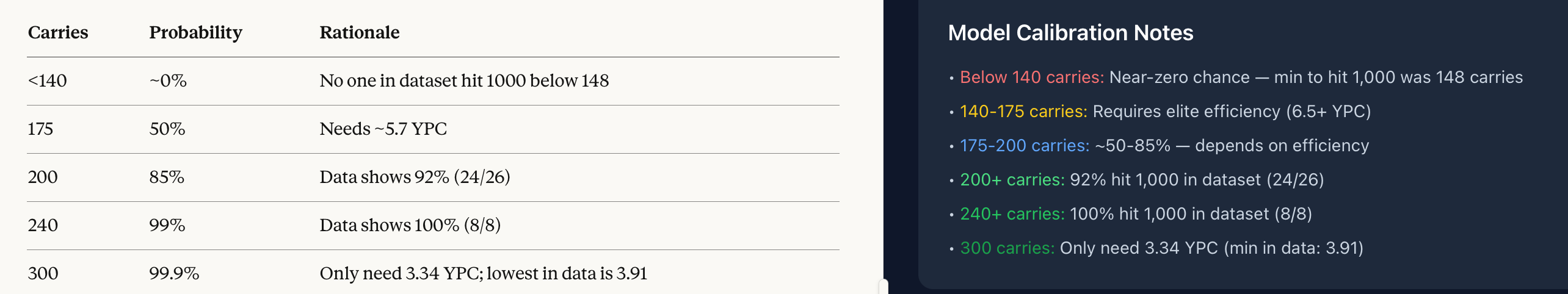
The function is using a normal (unconditional) way to come up with the probability measure. Because the sample size of players at various carry levels is small (for example, only 26 with 200 or more carries in 2025), the model probability is not set to match the exact frequency of occurrences in that group (200 carries suggests 85% probability to hit 1000 yards, yet 92% in sample achieved this).
Some data fudging is involved as an attempt to generalize away from the small sample size—to illustrate the point: just because 92% of the 26 players with 200+ carries hit 1000 yards in 2025, it doesn’t mean that this is the true probability generally speaking.
This is a hand wavy and haphazard way to go about things, but look, I’ve got things to do and it was a quick and easy method to solve a minor issue.
BTW, I know a lot of you out there are complaining about ‘polar vortexes’ and what not… here’s what I say: don’t run from it, embrace it. Winter is the season for the bold and the brave. The adventurers and explorers… ◾
PROBABILITY FUNCTION CODE
export default function RushingProbabilityCalculator() {
  const [carries, setCarries] = useState(150);

  const stats = useMemo(() => {
    // Calculate yards per carry distribution
    const ypcValues = rushingData.map(([c, y]) => y / c);
    const avgYpc = ypcValues.reduce((a, b) => a + b, 0) / ypcValues.length;
    const ypcStdDev = Math.sqrt(
      ypcValues.reduce((sum, ypc) => sum + Math.pow(ypc - avgYpc, 2), 0) / ypcValues.length
    );

    // Players who hit 1000 yards
    const hit1000 = rushingData.filter(([c, y]) => y >= 1000);
    const minCarries1000 = Math.min(...hit1000.map(([c]) => c));

    return { avgYpc, ypcStdDev, minCarries1000, hit1000Count: hit1000.length };
  }, []);

  const probability = useMemo(() => {
    // Calibrated from actual data:
    // - Below 140 carries: near-zero (min in dataset to hit 1000 was 148)
    // - 200+ carries: 92% hit 1000 (24/26)
    // - 240+ carries: 100% hit 1000 (8/8)
    // - At 300 carries, need only 3.34 YPC (min YPC in dataset is 3.91)

    // Hard floor: below 140 carries, virtually impossible
    if (carries < 140) {
      const prob = Math.max(0, 0.05 * Math.exp(-0.15 * (140 - carries)));
      return Math.round(prob * 1000) / 10;
    }

    // Piecewise linear interpolation based on actual data points:
    // 140 carries: ~5% (need elite 7.1+ YPC)
    // 175 carries: ~50% (need 5.7 YPC)
    // 200 carries: ~85% (based on data: some miss at 4.0-4.9 YPC)
    // 240 carries: ~99% (all 8 players in data hit it)
    // 300 carries: ~99.9% (need only 3.34 YPC, min in data is 3.91)

    let prob;
    if (carries < 175) {
      // 140-175: ramp from 5% to 50%
      prob = 0.05 + (0.45 * (carries - 140) / 35);
    } else if (carries < 200) {
      // 175-200: ramp from 50% to 85%
      prob = 0.50 + (0.35 * (carries - 175) / 25);
    } else if (carries < 240) {
      // 200-240: ramp from 85% to 99%
      prob = 0.85 + (0.14 * (carries - 200) / 40);
    } else {
      // 240+: asymptotic approach to 100%
      // At 240: 99%, at 300: 99.9%
      prob = 0.99 + (0.009 * Math.min(1, (carries - 240) / 60));
    }

    return Math.round(prob * 1000) / 10;
  }, [carries]);

  // Find comparable players from dataset
  const comparables = useMemo(() => {
    return rushingData
      .map(([c, y], i) => ({ carries: c, yards: y, hit1000: y >= 1000 }))
      .filter(p => Math.abs(p.carries - carries) <= 20)
      .sort((a, b) => Math.abs(a.carries - carries) - Math.abs(b.carries - carries))
      .slice(0, 5);
  }, [carries]);

  const getConfidenceColor = (prob) => {
    if (prob < 20) return 'text-red-600';
    if (prob < 40) return 'text-orange-500';
    if (prob < 60) return 'text-yellow-600';
    if (prob < 80) return 'text-green-500';
    return 'text-green-600';
  };

  const getConfidenceLabel = (prob) => {
    if (prob < 5) return 'Extremely Unlikely';
    if (prob < 20) return 'Very Unlikely';
    if (prob < 40) return 'Unlikely';
    if (prob < 60) return 'Possible';
    if (prob < 80) return 'Likely';
    if (prob < 95) return 'Very Likely';
    return 'Near Certain';
  };

  return (
    <div className="min-h-screen bg-slate-900 text-white p-6">
      <div className="max-w-2xl mx-auto">
        <h1 className="text-3xl font-bold text-center mb-2">
          1,000 Yard Rusher Probability
        </h1>
        <p className="text-slate-400 text-center mb-8">
          Based on 2025 college football rushing leaders
        </p>

        <div className="bg-slate-800 rounded-xl p-6 mb-6">
          <label className="block text-sm font-medium text-slate-300 mb-2">
            Projected Carries
          </label>
          <input
            type="range"
            min="50"
            max="320"
            value={carries}
            onChange={(e) => setCarries(Number(e.target.value))}
            className="w-full h-2 bg-slate-700 rounded-lg appearance-none cursor-pointer accent-blue-500"
          />
          <div className="flex justify-between mt-2">
            <span className="text-slate-500 text-sm">50</span>
            <span className="text-2xl font-bold text-blue-400">{carries}</span>
            <span className="text-slate-500 text-sm">320</span>
          </div>
        </div>

        <div className="bg-slate-800 rounded-xl p-6 mb-6 text-center">
          <p className="text-slate-400 text-sm mb-1">Probability of 1,000+ Rushing Yards</p>
          <p className={`text-6xl font-bold ${getConfidenceColor(probability)}`}>
            {probability}%
          </p>
          <p className={`text-lg mt-2 ${getConfidenceColor(probability)}`}>
            {getConfidenceLabel(probability)}
          </p>
        </div>

        <div className="bg-slate-800 rounded-xl p-6 mb-6">
          <h2 className="text-lg font-semibold mb-3">Model Calibration Notes</h2>
          <ul className="text-slate-300 text-sm space-y-2">
            <li>• <span className="text-red-400">Below 140 carries:</span> Near-zero chance — min to hit 1,000 was 148 carries</li>
            <li>• <span className="text-yellow-400">140-175 carries:</span> Requires elite efficiency (6.5+ YPC)</li>
            <li>• <span className="text-blue-400">175-200 carries:</span> ~50-85% — depends on efficiency</li>
            <li>• <span className="text-green-400">200+ carries:</span> 92% hit 1,000 in dataset (24/26)</li>
            <li>• <span className="text-green-500">240+ carries:</span> 100% hit 1,000 in dataset (8/8)</li>
            <li>• <span className="text-green-600">300 carries:</span> Only need 3.34 YPC (min in data: 3.91)</li>
          </ul>
        </div>

        {comparables.length > 0 && (
          <div className="bg-slate-800 rounded-xl p-6">
            <h2 className="text-lg font-semibold mb-3">
              Similar Carry Counts in Dataset
            </h2>
            <div className="space-y-2">
              {comparables.map((p, i) => (
                <div
                  key={i}
                  className={`flex justify-between p-2 rounded ${
                    p.hit1000 ? 'bg-green-900/30' : 'bg-red-900/30'
                  }`}
                >
                  <span>{p.carries} carries</span>
                  <span className="font-medium">
                    {p.yards} yds {p.hit1000 ? '✓' : '✗'}
                  </span>
                </div>
              ))}
            </div>
            <p className="text-slate-500 text-xs mt-3">
              Players within ±20 carries of your input
            </p>
          </div>
        )}

        <div className="mt-6 text-center text-slate-500 text-xs">
          Data: Top 100 rushers by yardage, 2025 season
        </div>
      </div>
    </div>
  );
}I would like to do an analysis in the near future studying player efficiency at different workload levels. A question that comes to mind is: how much of the player pool will degrade in performance (measured by YPC) after 20 carries per game… how many at 25… how many at 30? And who are the players who withstand heavy workload levels the best?
In a hypothetical study where we have all the complete data going years back, would Derrick Henry, who I think is the Ne Plus Ultra of workhorses, be the #1 player in the model in terms of maintaining consistent efficiency at each workload threshold (20, 25, 30…)? And then at what carry number would his efficiency begin to suffer? Unfortunately, it would be impossible to complete this type of analysis because the input data that this requires doesn’t exist.
Instead, I’m thinking I will need to generalize to a season-workload focus, and study players based on their first 50 carries, then their second 50 carries, up to 300 or 350, whichever the max is that season and ask the same question.
Unfortunately, small sample size at the higher end of the distribution would limit the scope of the model. For example, there may only be one player who sees more than 300 carries next season.